Examples

Basic functionalities

First of all import PyOphidia modules

from PyOphidia import cube, client

As a first command we need to connect to the Ophidia server front-end to load the modules variables and start an analytics session. So, we instantiate a new Client common to all Cube instances using setclient method (connection details are inferred from the environment with read_env=true).

cube.Cube.setclient(read_env=True)

Let’s now load a NetCDF file. We can inspect the file with the explorenc Ophidia operator that shows: - Dimension list: it contains the NetCDF file dimensions and their size; - Variable list: it includes the NetCDF file variables, their type and the related dimensions; - Metadata list: it shows file attributes

cube.Cube.explorenc(
         src_path="/home/ophidia/notebooks/tasmax_day_CMCC-CESM_rcp85_r1i1p1_20960101-21001231.nc"
     )

We can now create a datacube from a CMIP5 NetCDF (.nc) dataset produced by CMCC Foundation with the CESM model using the importnc operator with the following parameters: - src_path: contains the file path /home/ophidia/notebooks/tasmax_day_CMCC-CESM_rcp85_r1i1p1_20960101-21001231.nc - `measure='tasmax'`: it represents the variable to be imported (tasmax) - `imp_dim='time'`: it means that data should be arranged in order to operate on time series - ncores: it is the number of cores to be used - nfrag: it is the number of fragments - description: it represents the description associated to the datacube

Note: We are not directly reading the file content from the notebook

Single core: Import the input NetCDF file using 1 core and 4 fragments

tasmaxCube = cube.Cube.importnc2(
         src_path='/home/ophidia/notebooks/tasmax_day_CMCC-CESM_rcp85_r1i1p1_20960101-21001231.nc',
         measure='tasmax',
         imp_dim='time',
         ncores=1,
         nfrag=4,
         description="Imported cube (1 core)"
     )

Multi-core: Import the input NetCDF file using 4 cores and 4 fragments. This time the operator will run the import with 4 parallel processes and the execution time should take less.

tasmaxCube = cube.Cube.importnc2(
         src_path='/home/ophidia/notebooks/tasmax_day_CMCC-CESM_rcp85_r1i1p1_20960101-21001231.nc',
         measure='tasmax',
         imp_dim='time',
         ncores=4,
         nfrag=4,
         description="Imported cube (4 cores)",
     )

Check the datacubes available in the virtual file system. Ophidia manages a virtual file system associated with each user that provides a hierarchical organization of concepts, supporting:

• datacubes, the actual objects containing the data and related metadata;

• containers, grouping together a set of related datacubes;

• virtual folders, to store one or more containers according to the user’s needs.

In particular, we can use the list operator with the level of verbosity parameter (`level=2` shows folders, containers and datacubes)

cube.Cube.list(level=2)

To get the list of arguments and default values the python help() command can be used

help(cube.Cube)

Inspect the cube and its dimensions structure using the info() method. Note the data fragmentation table

tasmaxCube.info()

Subset the datacube over space (lat and lon) and time specifying `subset_dims="lat|lon|time"`. A filter with the actual dimension values (e.g `subset_filter="-50:20|20:160|JJA"`) can be provided using `subset_type="coord"`.

Note: each instance method produces a new datacube object

tasmaxCube2 = tasmaxCube.subset(
         subset_dims="lat|lon|time",
         subset_filter="-50:20|20:160|JJA",
         subset_type="coord",
         time_filter="yes",
         ncores=2,
         description="Subsetted cube"
     )

Inspect the new cube: the dimension sizes and fragmentation info have changed

tasmaxCube2.info()

But what does the datacube actually contain at this point? We can use the explore method to check the content. The `limit_filter=1` option allows to show only one row.

tasmaxCube2.explore(limit_filter=1)

We can also explore just a specific portion of the datacube. The explore operator supports filters on multiple dimensions similarly to the subset method. `subset_type="index"` allows to filter on dimension index.

tasmaxCube2.explore(subset_dims="lat|lon|time",subset_type="index",subset_filter="1:2|1:4|1:4")

Let’s compute the maximum value over the time series for each point in the spatial domain using `operation='max'`. We can also compute other metrics (see the documentation of OPH_REDUCE_).

tasmaxCube3 = tasmaxCube2.reduce(
                 operation='max',
                 ncores=2,
                 description="Reduced cube"
             )

In the new cube the time dimension is “collapsed” (size: ALL)

tasmaxCube3.info()

Note: Each operation executed creates a new datacube on the framework (datacubes are not overwritten)

cube.Cube.list(level=2)

Let’s export the data into a Python-friendly structure with the export_array() method.

Note: this is the first time we move data from the server-side to the Notebook

data = tasmaxCube3.export_array()
data

The structure looks something like this

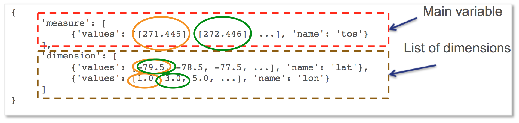
The data exported in the Python structure can be used to create a map with Cartopy and Matplolib (note the definition of a Python function)

%matplotlib inline

def plotData(data):

   import cartopy.crs as ccrs
   import matplotlib.pyplot as plt
   from cartopy.mpl.geoaxes import GeoAxes
   from cartopy.util import add_cyclic_point
   import numpy as np
   import warnings
   warnings.filterwarnings("ignore")

   fig = plt.figure(figsize=(12, 6), dpi=100)

   #Add Geo axes to the figure with the specified projection (PlateCarree)
   projection = ccrs.PlateCarree()
   ax = plt.axes(projection=projection)

   #Draw coastline and gridlines
   ax.coastlines()

   gl = ax.gridlines(crs=projection, draw_labels=True, linewidth=1, color='black', alpha=0.9, linestyle=':')
   gl.xlabels_top = False
   gl.ylabels_right = False

   lat = data['dimension'][0]['values'][ : ]
   lon = data['dimension'][1]['values'][ : ]
   var = data['measure'][0]['values'][ : ]
   var = np.reshape(var, (len(lat), len(lon)))

   #Wraparound points in longitude
   var_cyclic, lon_cyclic = add_cyclic_point(var, coord=np.asarray(lon))
   x, y = np.meshgrid(lon_cyclic,lat)

   #Define color levels for color bar
   clevs = np.arange(200,340,5)

   #Set filled contour plot
   cnplot = ax.contourf(x, y, var_cyclic, clevs, transform=projection,cmap=plt.cm.jet)
   plt.colorbar(cnplot,ax=ax)

   #Set the aspect of the axis scaling
   ax.set_aspect('auto', adjustable=None)

   plt.title('Maximum Near-Surface Air Temperature (deg K)')
   plt.show()

plotData(data)

We can save the results in a NetCDF file using the exportnc operator with the following parameters: - output_path: represents the destination path (/home/ophidia/notebooks/) - output_name: is the name of the output NetCDF file

tasmaxCube3.exportnc2(
     output_path="/home/ophidia/notebooks/",
     output_name='max'
)

What If we want to consider the whole spatial domain and specify a subset only on the time range?

We can perform the new set of operations on mycube object, without the need to re-import the dataset from the file. The time range can be provided in human-readable form with a datetime format (e.g `subset_filter="2096-01-01_2097-01-01"`) setting `time_filter="yes"`.

tasmaxCube2 = tasmaxCube.subset(
             subset_dims="time",
             subset_filter="2096-01-01_2096-12-31",
             subset_type="coord",
             time_filter="yes",
             ncores=2,
             description="New subsetted cube"
     )

tasmaxCube2.info()

We can rerun the same operation on the new cube …

tasmaxCube3 = tasmaxCube2.reduce(
             operation='max',
             ncores=2,
             description="New reduced cube"
         )

… and plot the new datacube values on a map using the function plotData

data = tasmaxCube3.export_array()
plotData(data)

What if we want to get the minimum instead of the maximum value?

Again we can apply the reduce operator with `operation='min'` on newMycube2 object, without the need to re-import or subset the dataset again

tasmaxCube3 = tasmaxCube2.reduce(
                 operation='min',
                 ncores=2,
                 description="New reduced cube2"
             )

… and plot the new datacube values on a map using the function plotData

data = tasmaxCube3.export_array()
plotData(data)

Now, we can import the NetCDF file for the tasmin variable…

tasminCube = cube.Cube.importnc2(
         src_path='/home/ophidia/notebooks/tasmin_day_CMCC-CESM_rcp85_r1i1p1_20960101-21001231.nc',
         measure='tasmin',
         imp_dim='time',
         ncores=4,
         nfrag=4,
         description="Imported cube"
     )

We can use the *predicate* evaluation operation into the apply operator in order to identify the days with temperature over a given threshold, e.g. 293.15°K (see the documentation of OPH_PREDICATE_).

Basically, we put to 1 the temperatures over 293.15°K (20°C), 0 otherwise.

tasminCube2 = tasminCube.apply(
   query="oph_predicate('OPH_FLOAT','OPH_INT',measure,'x-293.15','>0','1','0')",
   ncores=4
)
tasminCube2.info()

and count days over the given threshold on yearly basis. This is known as the Tropical Nights index: starting from the daily minimum temperature (2096-2100) TN, the Tropical Nights index is the number of days where $TN > T$ (T is a reference temperature, e.g. 20°C).

tropicalNights = tasminCube2.reduce2(
   operation='sum',
   dim='time',
   concept_level='y',
   ncores=4
)
tropicalNights.info()

Now, we can use the to_dataset method in order to export the datacube into an Xarray dataset.

tropicalNights_ds = tropicalNights.to_dataset().transpose('time','lat','lon')

We can explore the result that consists of the tasmin variable, coordinates and attributes which together form a self describing dataset (see the documentation of xarray.Dataset_)

tropicalNights_ds

Let’s plot all years from the dataset using Matplotlib and Cartopy. Basically, it is the same code of the plotData function with in addition the animation function that allows to flow the maps over years.

%matplotlib inline
import matplotlib as mpl
import matplotlib.pyplot as plt
import cartopy.crs as ccrs
from cartopy.mpl.geoaxes import GeoAxes
from cartopy.util import add_cyclic_point
from IPython.display import HTML
import matplotlib.animation as animation
import numpy as np
import warnings
import pandas as pd
warnings.filterwarnings("ignore")

def drawmap(ax,x,y,var_cyclic, clevs, title):
   ax.set_title(title, fontsize=14)
   projection = ccrs.PlateCarree()
   #Draw coastline and gridlines
   ax.coastlines()
   gl = ax.gridlines(crs=projection, draw_labels=True, linewidth=1, color='black', alpha=0.9, linestyle=':')
   gl.xlabels_top = False
   gl.ylabels_right = False
   #Set filled contour plot
   cs = ax.contourf(x, y, var_cyclic, clevs, cmap=plt.cm.Oranges)
   return cs

def myanimate(i, ax, dataset, values, lat, lon, x, y, var_cyclic, clevs):
   from datetime import datetime
   ax.clear()
   # change var_cyclic...
   var = values[i]
   var = np.reshape(var, (len(lat), len(lon)))
   #Wraparound points in longitude
   var_cyclic, lon_cyclic = add_cyclic_point(var, coord=np.asarray(lon))
   x, y = np.meshgrid(lon_cyclic,lat)
   year = datetime.fromisoformat(dataset['time'].values[i]).year
   new_contour = drawmap(ax,x,y,var_cyclic, clevs, year)
   return new_contour


def plotData(dataset):
   lat = dataset['lat'].values
   lon = dataset['lon'].values
   values = dataset['tasmin'].values
   max=dataset.tasmin.max()
   min=dataset.tasmin.min()

   fig = plt.figure(figsize=(12, 6), dpi=100)

   #Add Geo axes to the figure with the specified projection (PlateCarree)
   projection = ccrs.PlateCarree()
   ax = plt.axes(projection=projection)

   #Draw coastline and gridlines
   ax.coastlines()
   gl = ax.gridlines(crs=projection, draw_labels=True, linewidth=1, color='black', alpha=0.9, linestyle=':')
   gl.xlabels_top = False
   gl.ylabels_right = False

   var = values[0]
   var = np.reshape(var, (len(lat), len(lon)))

   #Wraparound points in longitude
   var_cyclic, lon_cyclic = add_cyclic_point(var, coord=np.asarray(lon))
   x, y = np.meshgrid(lon_cyclic,lat)

   #Define color levels for color bar
   levStep = (max-min)/20
   clevs = np.arange(min,max+levStep,levStep)

   #Set filled contour plot
   first_contour = drawmap(ax,x,y,var_cyclic, clevs, dataset['time'].values[0])

   #Make a color bar
   plt.colorbar(first_contour, fraction=0.047*0.493)

   #Set the aspect of the axis scaling
   ax.set_aspect('auto', adjustable=None)

   plt.close(fig)

   #Execute the myanimate function that change maps over time
   ani = animation.FuncAnimation(fig, myanimate, fargs=(ax, dataset, values, lat, lon, x, y, var_cyclic, clevs), frames=np.arange(5), interval=500)
   return HTML(ani.to_jshtml())

plotData(tropicalNights_ds)

Time series processing

Starting from the first imported datacube, we can extract a single time series for a given spatial point

tasmaxCube2 = tasmaxCube.subset(
         subset_dims="lat|lon|time",
         subset_filter="42|15|2096-01-01_2096-12-31",
         subset_type="coord",
         ncores=2,
         time_filter="yes",
         description="Subsetted cube"

)

Then compute the moving average on each element of the measure array using the apply operator with the oph_moving_avg primitive (see the documentation of OPH_MOVING_AVG_).

Note: the moving average is defined as an average of fixed number of items in the time series

movingAvg = tasmaxCube2.apply(
   query="oph_moving_avg('OPH_FLOAT','OPH_FLOAT',measure,7.0,'OPH_SMA')"
)

We export the datacubes into Xarray datasets…

tasmaxCube2_ds = tasmaxCube2.to_dataset()
tasmaxCube2_ds

movingAvg_ds = movingAvg.to_dataset()
movingAvg_ds

…and plot the two time series (tasmaxCube2_ds and movingAvg_ds) using the Bokeh Visualization library (see Bokeh_).

from datetime import datetime, timedelta
from bokeh.plotting import figure, output_notebook, show
from bokeh.models import ColumnDataSource, Legend, DatetimeTickFormatter, DatetimeTicker, Range1d, HoverTool
labels = []
for t in tasmaxCube2_ds['time'].values:
   labels.append(datetime.strptime(str(t).split(" ")[0], '%Y-%m-%d'))
# Set ColumnDataSource for each metric
source_metrics = {'time': labels, '2096': tasmaxCube2_ds.tasmax.values.flatten(),
                 'moving_avg': movingAvg_ds.tasmax.values.flatten()}
source = ColumnDataSource(data = source_metrics)
# Create the right number of ticks on the x axis so as not to make them overlap
date_values = []
start_date = labels[0]
end_date = labels[-1]
delta = timedelta(days=1)
while start_date <= end_date:
   date_values.append(start_date)
   start_date += delta
if len(date_values)>50:
   number_ticks = 50
else:
   number_ticks = len(date_values)
# Create figure and time series:
p = figure(x_axis_type = 'datetime', y_axis_label = 'tasmax (degK)',
          plot_height=400, plot_width=950, title="Maximum Near-Surface Air Temperature")

r1 = p.line(x='time', y='2096', line_width=2, color="#ff66cc", source=source)
r2 = p.line(x='time', y='moving_avg', line_width=2, color="#00cc99", source=source)

# Set legend
legend = Legend(items=[("2096", [r1]), ("moving_avg", [r2])], location="top_right")
p.add_layout(legend, 'right')
# Set some properties to make plot better
p.legend.click_policy="hide"
p.xgrid.grid_line_color = None
p.xaxis.axis_label = "Time"
p.xaxis.major_label_orientation = 1.2

# Format x axis
x_range = Range1d(labels[0].timestamp()*1000, labels[-1].timestamp()*1000)
p.x_range= x_range
p.xaxis.formatter=DatetimeTickFormatter(days="%Y-%m-%d", months="%Y-%m-%d", hours="%Y-%m-%d", minutes="%Y-%m-%d")
p.xaxis.ticker = DatetimeTicker(desired_num_ticks=number_ticks)

# Add hover tooltip
p.add_tools(HoverTool(
   tooltips=[
       ( 'time',  '@time{%F}'   ),
       ( '2096',  '@2096' ),
       ( 'moving_avg', '@moving_avg'),
   ],
   formatters={'@time': 'datetime'},
   mode='vline',
   renderers=[r1]
))
output_notebook()
show(p)

Compare two time series.

We can also compute the difference between two time series (also from different cubes).

Let’s first compute the monthly average over the time series using the reduce2 operator with `operation='avg'` and `concept_level='M'`.

avgCube = tasmaxCube.reduce2(
   operation='avg',
   dim='time',
   concept_level='M',
)

Extract the first time series (2096) using the subset operator with fixed latitude and longitude.

firstYear = avgCube.subset(
             subset_dims="lat|lon|time",
             subset_type="coord",
             subset_filter="42|15|2096-01-01_2096-12-31",
             ncores=2,
             time_filter="yes",
             description="Subsetted cube (2096)"
         )

In the same way, extract the second time series (2097)

secondYear = avgCube.subset(
             subset_dims="lat|lon|time",
             subset_type="coord",
             subset_filter="42|15|2097-01-01_2097-12-31",
             ncores=2,
             time_filter="yes",
             description="Subsetted cube (2097)"
         )

We can check the structure for the 2nd cube

secondYear.info()

Compute the difference between 2097 and 2096 monthly-mean time series. The intercube operator provides other types of inter-cube operations (http://ophidia.cmcc.it/documentation/users/operators/OPH_INTERCUBE.html)

diffCube = secondYear.intercube(cube2=firstYear.pid,operation="sub")

Export the datacube into a dataset structure

diffCube_ds = diffCube.to_dataset()
diffCube_ds

and finally plot the result with Bokeh library

values = diffCube_ds.tasmax.values
months = ["Jan", "Feb", "Mar", "Apr", "May", "Jun", "Jul", "Aug", "Sep", "Oct", "Nov", "Dec"]
source_metrics = {'time': months, 'values': values.flatten()}
source = ColumnDataSource(data = source_metrics)
p1 = figure(x_range = months, y_axis_label = 'tasmax difference (degC)', plot_height=400, plot_width=950,
           title="Maximum Near-Surface Air Temperature - difference 2097-2096")
v = p1.vbar(x='time', top='values', width=0.3, source=source)
# Set some properties to make plot better
p1.xaxis.axis_label = "Time"
p1.xaxis.major_label_orientation = 1.2
p1.xaxis.major_label_text_font_size="13px"
# Add hover tooltip
p1.add_tools(HoverTool(
   tooltips=[
       ( 'month',  '@time'   ),
       ( 'difference',  '@values' ),
   ],
   mode='vline',
   renderers=[v]
))
output_notebook()
show(p1)

Our workspace now contains several datacubes from the experiments just run.

cube.Cube.list(level=2)

Once done, we can clear the space before moving to other notebooks using the deletecontainer method with the container name (e.g `container='tasmax_day_CMCC-CESM_rcp85_r1i1p1_20960101-21001231.nc'`).

cube.Cube.deletecontainer(container='tasmax_day_CMCC-CESM_rcp85_r1i1p1_20960101-21001231.nc',force='yes')
cube.Cube.deletecontainer(container='tasmin_day_CMCC-CESM_rcp85_r1i1p1_20960101-21001231.nc',force='yes')

The virtual file system should now be “clean”

cube.Cube.list(level=2)